Deep Phenotyping of Maternal Trajectories Among Pregnant Women in Cape Town, South Africa Using K-means Clustering
Data
Identifying the drinking/smoking patterns of women during pregnancy is important in order to better understand the risk of possible postnatal outcomes.
For this project, I analyzed data from a multi-center, prospective pregnancy cohort study that collected data from women living in Cape Town, South Africa. This population is at high risk for drinking and smoking during pregnancy. The goal of the study was to investigate how prenatal drinking, prenatal smoking, and emotional state during pregnancy may effect postnatal outcomes - specifically child heart rate during third trimester, gestational age in weeks, and baby weight at birth (in pounds). I conducted exploratory analysis to identify trends and associations.
Some participants did not have available data for all three trimesters. For this analysis, only those who did have all trimester data available were included.
Clustering
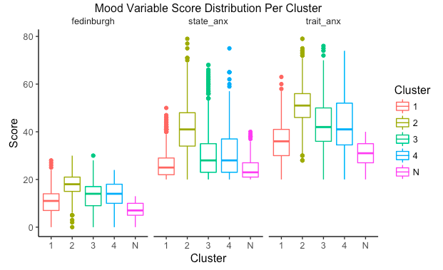
Since the women demonstrate dynamic drinking and smoking habits, the first step was to define the exposure variable by clustering the women based on their drinking and smoking patterns. I accomplished this through the use of k-means clustering. There is also depression and anxiety data available for the women. At the beginning of the study, each participant was given the fedinburgh depression scale questionnaire and a depression score was calculated. They were also given the State-Trait Anxiety Inventory (STAI), a psychological inventory based on a 4-point scale that consists of 40 questions on a self-report basis. The STAI measures two types of anxiety – state anxiety, or anxiety about an event, and trait anxiety, or anxiety level as a personal characteristic. There is the possibility of an association between smoking, drinking, depression, and anxiety. It was decided to use the five variables to cluster the women. The variables used to cluster are
- Total Cigarettes Smoked Per Trimester
- Total Standard Drinks Per Trimester
- A “mood” variable made up of the women’s fedinburgh, state anxiety, and trait anxiety scores
The data is longitudinal, and therefore I used the ‘kml3d’ package in R to create trajectories. The kml3d package is “an implementation of k-means specifically designed to cluster joint trajectories (longitudinal data on several variable-trajectories)”. Further details about the package can be found here.
Prior to clustering, we wanted to establish a “non-exposed” group. Therefore, those who did not drink or smoke throughout their pregnancy were considered non-exposed and were not included in the clustering. 13 is the cut off score for the fedinburgh depression variable, and for 40 the state and trait anxiety variables. Those below the cut off are non-exposed (i.e not depressed). There are 154 subjects who are missing at least one mood variable (either state anxiety, trait anxiety, or fedinburgh). Those subjects were removed from clustering. I included sample code for both the clusters and the visualization of variables per cluster.
# Clustering
cld.joint.fedinburgh <- cld3d(pass.US.completers.fedinburgh[pass.US.completers.fedinburgh$Exposure ==
1,], timeInData = list(grep('TotCigsT',names(merge)),grep('TotalStdDrinksT',names(merge)),rep(181,
3)), time = c(1,2,3))
kml3d(cld.joint.fedinburgh,nbClusters = 4:9)
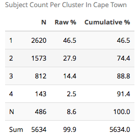
The sample size table is as follows:
Number of clusters
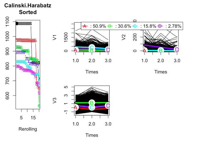
The Calinski & Harabasz criteria was used to choose the number of clusters. The following plots show the longitudinal trajectories for each set of variables for a given cluster size. From this criteria, 4 clusters were used as the best number of clusters.
Visualizing The Clusters
ggplot(melt(pass.US.completers.fedinburgh[,c("patid","Cluster.TotalJoint",
cigvars)], id=c('patid','Cluster.TotalJoint')), aes(x=variable,y=value,
group=patid, colour=Cluster.TotalJoint)) +
ggtitle("Total Cigarettes for Joint Cluster") +
stat_summary(aes(y = value,group = Cluster.TotalJoint), fun.y=mean,
geom="line",size=2) +
scale_x_discrete(labels=c("T1","T2","T3")) +
facet_grid(. ~ Cluster.TotalJoint)
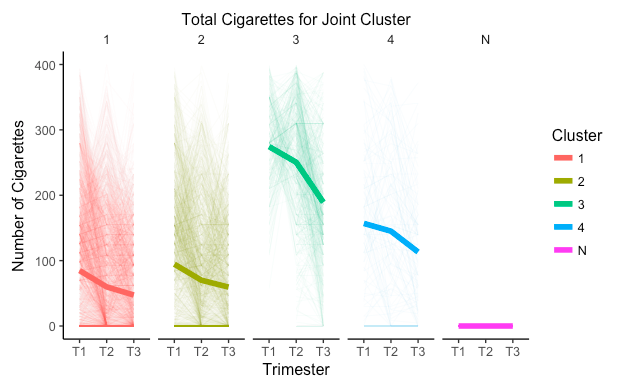
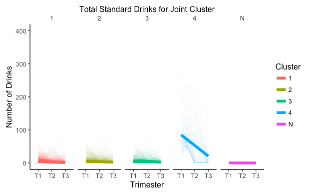
I have included descriptive statistics for the variables of interest stratified by cluster.
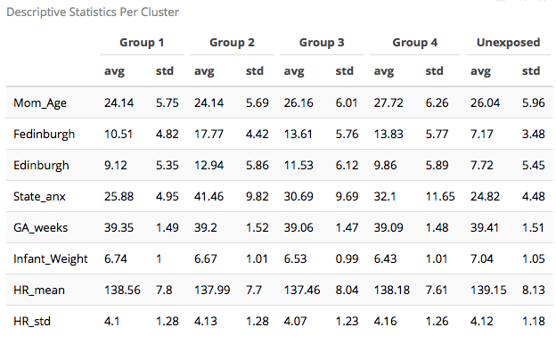
I defined the unexposed group (N) as those who did not smoke, did not drink, and did not experience any anxiety or depression during pregnancy. The clustering shows that cluster 1 is a low smoking, low alcohol consumption, and low depression group. Cluster 2 is a low alcohol consumption, moderate smoking, and high anxiety group. Cluster 3 is a low alcohol consumption, high smoking, and moderate anxiety group. Last, cluster 4 is the more severe group with high smoking, high alcohol consumption, and moderate anxiety and depression.
Visualizing Outcome Variables
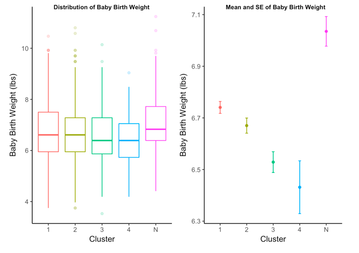
To visualize the outcomes per cluster, I began by creating boxplots of each outcome variable. This allows me to visually inspect the distribution and see if any major differences stand out.
To reiterate, the outcome variables being analyzed are:
- gestational age in weeks at birth
- child birth weight in pounds
- child heart rate in the third trimester


ANOVA Test for Differences
ANOVA analysis was done to evaluate any differences in the outcome variables between the clusters. The first step is to check the homogeneity of variance between the clusters using Levene’s test.
The null hypothesis for Levene’s test is that there is homogeneity of variance between the clusters versus the alternative that states there is no homogeneity of variance. None of the p-values were significant, and therefore we will assume homogeneity of variance.
I have included sample code.
library(car)

leveneTest(hrmean1 ~ Cluster.TotalJoint, data = outcome_set)

anova.hrmean <- aov(hrmean1 ~ Cluster.TotalJoint, data = outcome_set)

summary(anova.hrmean)
I included the ANOVA results for all outcome variables.

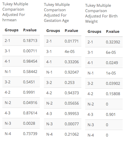
All three have p-values smaller than 0.05, therefore I used Tukey’s Multiple Comparison Correction to identify which clusters differ.
Heart Rate, Gestational Age, and Birth Weight
Heart Rate
For the third trimester heart rate, the differing clusters are:
- cluster 3 and 1
- unexposed and cluster 2
- unexposed and cluster 3
Gestational age
For the gestational age outcome, the differing clusters are:
- clusters 2 and 1
- clusters 3 and 1
- unexposed and cluster 3
Birth Weight
For the birth weight outcome, the differing clusters are:
- clusters 3 and 1
- clusters 4 and 1
- unexposed and cluster 1
- clusters 3 and 2
- unexposed and cluster 2
- unexposed and cluster 3
- unexposed and cluster 4
Summary
The goal is to identify wether there are different mean outcomes between the clusters and, specifically, the unexposed group. The unexposed group has a significantly higher heart rate mean than cluster 2, at an alpha level of 0.05, with a p-value of 0.04916. For gestational age, the unexposed group has a significantly higher gestational age in weeks than cluster 3, at an alpha level of 0.05, with a p-value of 0.00077. For birth weight, the unexposed group has a significantly higher birth weight than all four clusters, at an alpha level of 0.05. Although the analysis is exploratory, it seems that smoking and drinking may lead to changes in gestational age, birth weight, and heart rate.
Moving forward, I would like to explore a different number of clusters, specifically 5 and 6. The clusters may sparse out more and have a better clinical interpretation. The results also hint at signs of possible accelerated development. Accelerated development occurs when the baby begins to develop sooner than what is considered normal. The baby may show signs of a slower heart rate, increase in heart variability, and fast weight gain. This may be associated with preterm birth.
